线性网络

1 线性回归

1.1 数学建模

线性回归常见用在一些简单问题上（例如房价预测）

线性假设是指目标（房屋价格）可以表示为特征（面积和房龄）的加权和，如下面的式子：

$$ \mathrm{price} = w_{\mathrm{area}} \cdot \mathrm{area} + w_{\mathrm{age}} \cdot \mathrm{age} + b. $$

将式子总结一下可以写成线性代数结合权重的形式

$$ \hat{y} = w_1 x_1 + ... + w_d x_d + b $$

对于预测值（上方有尖括号）通过矩阵总结可以写成

$$ {\hat{\mathbf{y}}} = \mathbf{X} \mathbf{w} + b $$

随后就可以设置损失函数为平方误差

$$ l^{(i)}(\mathbf{w}, b) = \frac{1}{2} \left(\hat{y}^{(i)} - y^{(i)}\right)^2. $$

在多个样本上求平均值，可以列出

$$ L(\mathbf{w}, b) =\frac{1}{n}\sum_{i=1}^n l^{(i)}(\mathbf{w}, b) =\frac{1}{n} \sum_{i=1}^n \frac{1}{2}\left(\mathbf{w}^\top \mathbf{x}^{(i)} + b - y^{(i)}\right)^2. $$

1.2 解析解

在训练模型的时候我们希望寻找一组参数，这组参数能最小化在所有训练样本上的总损失。如下式：

$$ \mathbf{w}^*, b^* = \operatorname*{argmin}_{\mathbf{w}, b}\ L(\mathbf{w}, b). $$

通过数学推导我们其实是可以通过数学方式得到解析解的

$$ \mathbf{w}^* = (\mathbf X^\top \mathbf X)^{-1}\mathbf X^\top \mathbf{y}. $$

但是在机器学习中日后的问题都没有这么简单，问题也不一定会有解析解

1.3 代码实现

实际代码实现中要考虑很多的细节，具体可以参见 GitHub 链接

从零开始实现线性回归

使用 PyTorch 实现线性回归

2 Softmax 回归

2.1 Loss Function

这里列举了一些常用的损失函数

2.1.1 Cross Entropy

交叉熵损失，一般用来衡量概率之间的 loss，常用方法就是计算预测结果和实际结果之间的交叉熵

$ y $ 是 one-hot 标签，$\hat{y}$ 是 softmax 后得到的概率分布

$$ \mathcal{L} = - \sum_{i=1}^{C} y_i \log(\hat{y}_i) $$

因为 one-hot 只有一个位置是 1，其他的都是 0，所以可以直接简化为算目标结果的负对数

实际代码中我们常用一个运算操作来直接取出对应位置的预测值，第一维度是我们写的数值，第二维度是 y 实际数值

y = torch.tensor([0, 2])
y_hat = torch.tensor([[0.1, 0.3, 0.6], [0.3, 0.2, 0.5]])
y_hat[[0, 1], y] # tensor([0.1000, 0.5000])

# 计算负对数实现
def cross_entropy(y_hat, y):
    # 拿到真实数值
    num_label = range(len(y_hat))
    poss = y_hat[num_label, y] # 拿到真实数值的对应值
    return -torch.log(poss)

2.1.2 L2 Loss

就是差的平方，有时候会 /2 为了计算梯度

缺点是导数是一个线性的函数，离原点越远梯度越大

$$ \mathcal{L}_{L2}(y, \hat{y}) = \| y - \hat{y} \|_2^2 = \sum_{i=1}^{n} (y_i - \hat{y}_i)^2 $$

也有 平均格式，这个就是 MSE

$$ \mathcal{L}_{\text{MSE}} = \frac{1}{n}\sum_{i=1}^{n}(y_i - \hat{y}_i)^2 $$

2.1.3 L1 Loss

L1 Loss 就是绝对值之差，导数是正负 1

缺点是在零点处不可导

$$ \mathcal{L}_{L1}(y, \hat{y}) = \| y - \hat{y} \|_1 = \sum_{i=1}^{n} |y_i - \hat{y}_i| $$

2.1.4 Huber Loss

在大误差的时候使用 L1，小误差使用 L2，结合了两者的特点

$$ \mathcal{L}_{\delta}(y,\hat{y}) = \begin{cases} \frac{1}{2}(y-\hat{y})^2, & \text{if } |y-\hat{y}| \le \delta \\[6pt] \delta |y-\hat{y}| - \frac{1}{2}\delta^2, & \text{if } |y-\hat{y}| > \delta \end{cases} $$

2.2 代码实现

softmax 的主要特点是，每个元素都非负数，并且求和为 1，拥有概率的属性

$$ \text{softmax}(\mathbf{z})_i = \frac{\exp(z_i)}{\sum_{j=1}^{K} \exp(z_j)} $$

在代码的实现中使用了矩阵降维求和，这对于一个矩阵相当去把这个维度压缩到一起

def softmax(X):
    # softmax 核心： 分子 exp, 分母 exp并求和
    X_exp = torch.exp(X)
    partition = X_exp.sum(1, keepdim=True) # 对矩阵行进行求和
    return X_exp / partition # 使用了广播机制

实际的完整代码比较多，太长了就不放在这里了，可以 通过 GitHub 仓库查看

2.3 运行结果展示

<Figure size 700x500 with 1 Axes>
Epoch [1], Train loss 0.787, Test acc 0.748
<Figure size 700x500 with 1 Axes>
Epoch [2], Train loss 0.571, Test acc 0.812
<Figure size 700x500 with 1 Axes>
Epoch [3], Train loss 0.525, Test acc 0.826
<Figure size 700x500 with 1 Axes>
Epoch [4], Train loss 0.502, Test acc 0.832
<Figure size 700x500 with 1 Axes>
Epoch [5], Train loss 0.486, Test acc 0.837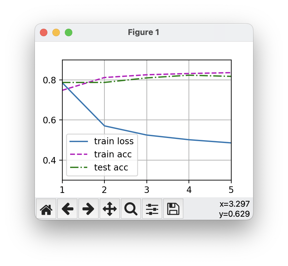

3 训练流程代码

里面有一些代码是比较通用的，主要是训练流程的编写代码，我认为还是有必要在这里展示的：

# 单个 epoch 的训练代码
def train_epoch_ch3(net, train_iter, loss, updater):  #@save
    """训练模型一个迭代周期（定义见第3章）"""
    # 将模型设置为训练模式
    if isinstance(net, torch.nn.Module):
        net.train()
    # 训练损失总和、训练准确度总和、样本数
    metric = Accumulator(3)
    for X, y in train_iter:
        # 计算梯度并更新参数
        y_hat = net(X)
        l = loss(y_hat, y)
        if isinstance(updater, torch.optim.Optimizer):
            # 使用PyTorch内置的优化器和损失函数
            updater.zero_grad()
            l.mean().backward()
            updater.step()
        else:
            # 使用定制的优化器和损失函数
            l.sum().backward()  # loss 求和并进行梯度运算
            updater(X.shape[0])
        
        # loss 取标量去除梯度
        metric.add(float(l.sum().item()), accuracy(y_hat, y), y.numel())
    # 返回训练损失和训练精度
    return metric[0] / metric[2], metric[1] / metric[2]

以及对外完整封装的训练代码

# 完整的训练代码
def train_ch3(net, train_iter, test_iter, loss, num_epochs, updater):  #@save
    """训练模型（定义见第3章）"""
    # 这是一个数据可视化的函数
    animator = d2l.Animator(xlabel='epoch', xlim=[1, num_epochs], ylim=[0.3, 0.9],
                        legend=['train loss', 'train acc', 'test acc'])
    for epoch in range(num_epochs):
        train_metrics = train_epoch_ch3(net, train_iter, loss, updater) # 训练一个 epoch
        test_acc = evaluate_accuracy(net, test_iter)    # 测试评估训练的结果
        animator.add(epoch + 1, train_metrics + (test_acc,))    # 绘制结果
        print(f"Epoch [{epoch + 1}], Train loss {train_metrics[0]:.3f}, Test acc {train_metrics[1]:.3f}")
    # train_loss, train_acc = train_metrics
    # d2l.plt.show() # 训练结果展示图片